An Introduction to glmtlp

Chunlin Li, Yu Yang, Chong Wu

October 02, 2024

Introduction

glmtlp fits generalized linear models via penalized maximum likelihood. It currently supports linear and logistic regression models. The regularization path is computed for the l0, l1, and TLP penalty at a grid of values for the regularization parameter lambda $\lambda$ (for l1 and TLP penalty) or kappa $\kappa$ (for l0 penalty). In addition, the package provides methods for prediction and plotting, and functions for cross-validation.

The authors of glmtlp are Chunlin Li, Yu Yang, and Chong Wu, and the R package is maintained by Chunlin Li and Yu Yang. A Python version is under development.

This vignette describes basic usage of glmtlp in R.

Installation

Install the package from CRAN.

install.packages("glmtlp")

Quick Start

In this section, we go over the main functions and outputs in the package.

First, we load the glmtlp package:

library(glmtlp)

We load a simulated data set with continuous response to illustrate the usage of linear regression.

data(gau_data)
X <- gau_data$X
y <- gau_data$y

We fit three models by calling glmtlp with X, y, family="gaussian" and three different penalty. The returned fit is an object of class glmtlp that contains all relevant information of the fitted model for further use. Users can apply plot, coef and predict methods to the fitted objects to get more detailed results.

fit <- glmtlp(X, y, family = "gaussian", penalty = "tlp")
fit2 <- glmtlp(X, y, family = "gaussian", penalty = "l0")
fit3 <- glmtlp(X, y, family = "gaussian", penalty = "l1")

We can visualize the coefficients and the solution path by executing the plot method. The output is a ggplot object. Therefore, the users are allowed to customize the plot to suit their own needs. The plot shows the solution path of the model, with each curve corresponding to a variable. Users may also choose to annotate the curves by setting label=TRUE. xvar is the index variable to plot against. Note that for “l1” or “tlp” penalty, xvar could be chosen from c("lambda", "log_lambda", "deviance", "l1_norm"), and for “l0” penalty, xvar could be chosen as "kappa".

plot(fit, xvar = "lambda")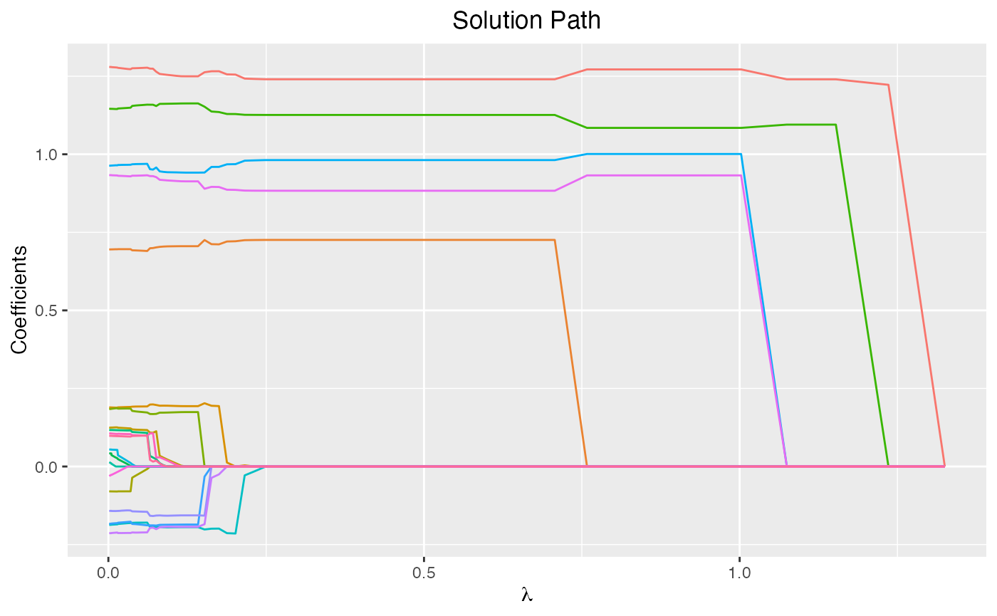

We can use the coef function to obtain the fitted coefficients. By default, the results would be a matrix, with each column representing the coefficients for every $\lambda$ or $\kappa$. The users may also choose to input the desired value of $\lambda$ or $\kappa$. Note that the user-supplied $\lambda$ or $\kappa$ parameter should be in the range of the parameter sequence used in the fitted model.

coef(fit)

...
##              1.32501    1.23571    1.15242     1.07475     1.00232     0.93477
## intercept -0.2428484 -0.1352757 -0.0235558 -0.02355059 -0.05190855 -0.05192106
## V1         0.0000000  1.2224980  1.2400538  1.24005913  1.27181076  1.27178077
## V2         0.0000000  0.0000000  0.0000000  0.00000000  0.00000000  0.00000000
## V3         0.0000000  0.0000000  0.0000000  0.00000000  0.00000000  0.00000000
## V4         0.0000000  0.0000000  0.0000000  0.00000000  0.00000000  0.00000000
## V5         0.0000000  0.0000000  0.0000000  0.00000000  0.00000000  0.00000000
## V6         0.0000000  0.0000000  0.0000000  0.00000000  0.93236905  0.93231995
## V7         0.0000000  0.0000000  0.0000000  0.00000000  0.00000000  0.00000000
## V8         0.0000000  0.0000000  0.0000000  0.00000000  0.00000000  0.00000000
...

coef(fit, lambda = 0.1)

...
##   intercept          V1          V2          V3          V4          V5 
##  0.03012329  1.25295108  0.00000000 -0.18639467 -0.15726983 -0.19310409 
##          V6          V7          V8          V9         V10         V11 
##  0.91543631  0.00000000  0.01275199  0.00000000  0.70521331  0.19432176 
##         V12         V13         V14         V15         V16         V17 
##  0.01640360  0.00000000  0.17320713  1.16204702  0.00000000  0.00000000 
##         V18         V19         V20 
##  0.00000000 -0.19471461  0.94229082
NA
NA
...

In addition, we can make predictions by applying the predict method. For this, users need to input a design matrix and the type of prediction to be made. Also, users can provide the desired level of regularization parameters or the indices of the parameter sequence. If neither is provided, then the prediction will be made for the whole lambda or kappa sequence.

predict(fit, X[1:5, ], lambda = 0.1)

## [1]  0.09972438  2.66195238 -1.33516956  0.33721013 -2.63615326

predict(fit, X[1:5, ], which = 10) # the 10th lambda in the lambda sequence

## [1]  0.1906092  2.2279251 -1.4255474  0.9313526 -2.8151620

Cross-validation can be implemented by cv.glmtlp to find the best regularization parameter. cv.glmtlp returns a cv.glmtlp object, a list with all the ingredients of the cross-validated fit. Users may use coef, predict, and plot to further check the cross-validation results.

cv.fit <- cv.glmtlp(X, y, family = "gaussian", penalty = "tlp")

The plot method will plot the deviance against the parameter sequence. The vertical dashed line shows the position of the index where the smallest CV error is achieved, and users may also choose to omit it by setting vertical.line = FALSE. Again, the output is a ggplot object, so users are free to make modifications to it.

plot(cv.fit)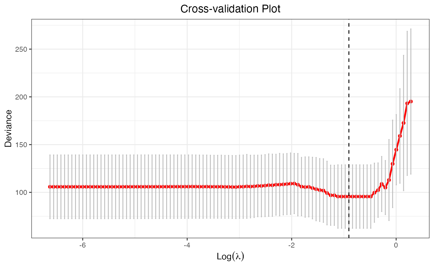

The coef and predict method by default use the parameter that gives the smallest CV error, namely, which = cv.fit$idx.min.

coef(cv.fit)

##    intercept           V1           V2           V3           V4           V5 
## -0.009695669  1.240195285  0.000000000  0.000000000  0.000000000  0.000000000 
##           V6           V7           V8           V9          V10          V11 
##  0.883162055  0.000000000  0.000000000  0.000000000  0.725706691  0.000000000 
##          V12          V13          V14          V15          V16          V17 
##  0.000000000  0.000000000  0.000000000  1.125977511  0.000000000  0.000000000 
##          V18          V19          V20 
##  0.000000000  0.000000000  0.981387932

predict(cv.fit, X[1:5, ])

## [1]  0.1906096  2.2279220 -1.4255447  0.9313487 -2.8151577

References

Li, C., Shen, X., & Pan, W. (2021). Inference for a large directed graphical model with interventions. arXiv preprint arXiv:2110.03805. https://arxiv.org/abs/2110.03805.

Shen, X., Pan, W., & Zhu, Y. (2012). Likelihood-based selection and sharp parameter estimation. Journal of the American Statistical Association, 107(497), 223-232. https://doi.org/10.1080/01621459.2011.645783.

Shen, X., Pan, W., Zhu, Y., & Zhou, H. (2013). On constrained and regularized high-dimensional regression. Annals of the Institute of Statistical Mathematics, 65(5), 807-832. https://doi.org/10.1007/s10463-012-0396-3.

Tibshirani, R., Bien, J., Friedman, J., Hastie, T., Simon, N., Taylor, J., & Tibshirani, R. J. (2012). Strong rules for discarding predictors in lasso‐type problems. Journal of the Royal Statistical Society: Series B (Statistical Methodology), 74(2), 245-266. https://doi.org/10.1111/j.1467-9868.2011.01004.x.

Yang, Y. & Zou, H. A coordinate majorization descent algorithm for l1 penalized learning. Journal of Statistical Computation and Simulation 84.1 (2014): 84-95. https://doi.org/10.1080/00949655.2012.695374.

Zhu, Y., Shen, X., & Pan, W. (2020). On high-dimensional constrained maximum likelihood inference. Journal of the American Statistical Association, 115(529), 217-230. https://doi.org/10.1080/01621459.2018.1540986.

Zhu, Y. (2017). An augmented ADMM algorithm with application to the generalized lasso problem. Journal of Computational and Graphical Statistics, 26(1), 195-204. https://doi.org/10.1080/10618600.2015.1114491.