Plot Method for a "glmtlp" Object
plot.glmtlp.RdGenerates a solution path plot for a fitted "glmtlp" object.
Arguments
- x
Fitted
glmtlpobject.- xvar
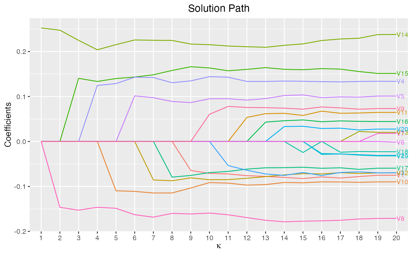
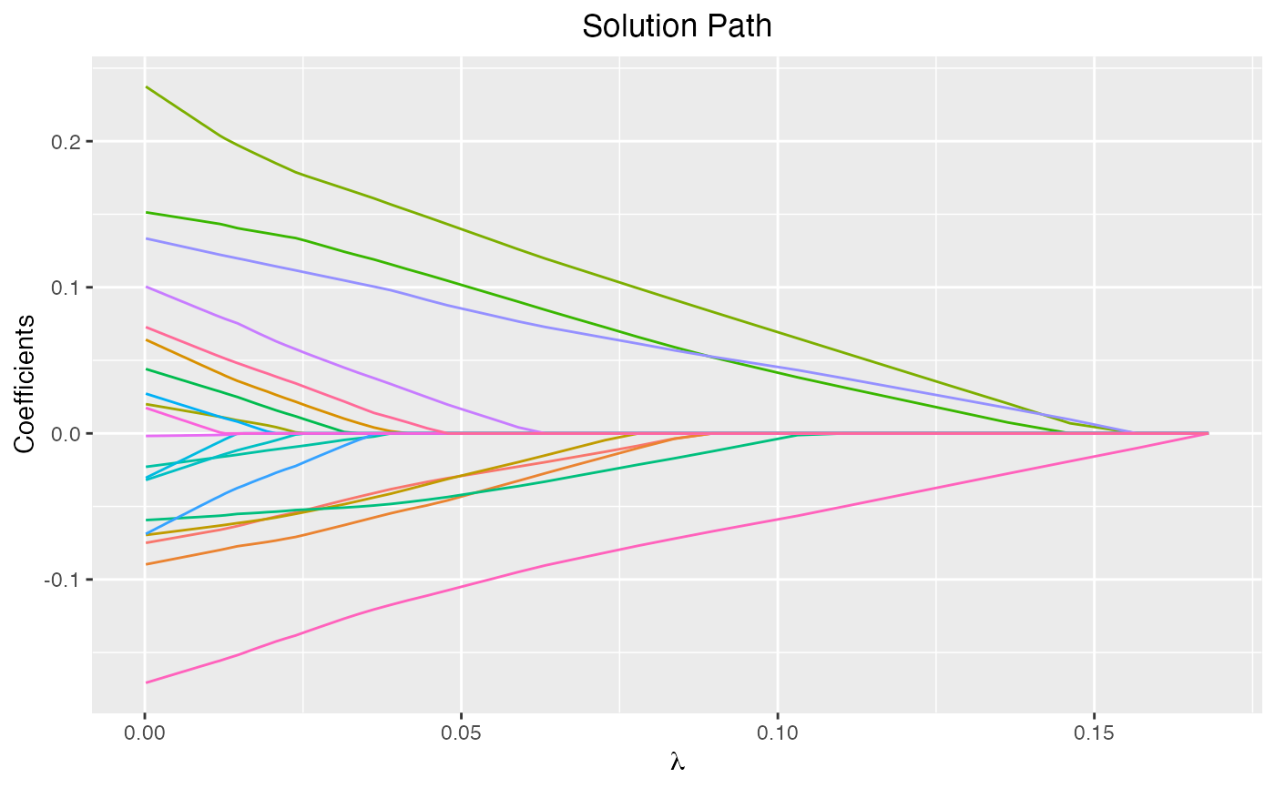
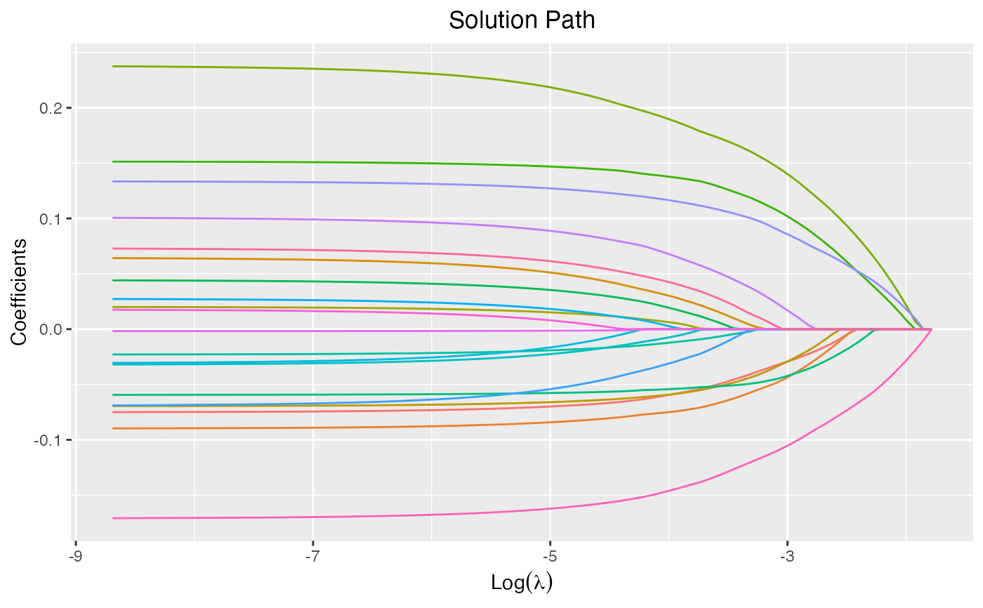
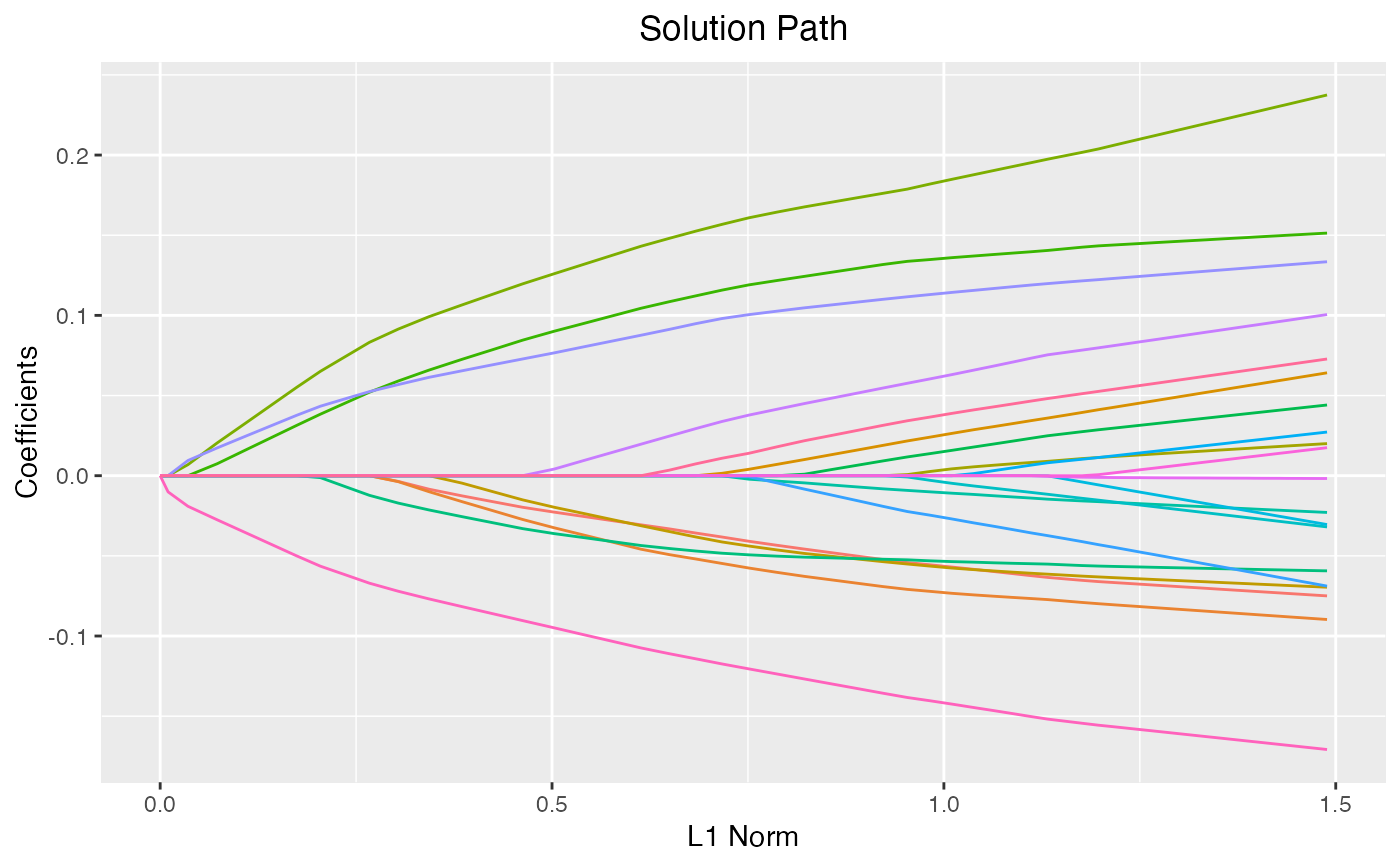
The x-axis variable to plot against, including
"lambda","kappa","deviance","l1_norm", and"log_lambda".- xlab
The x-axis label of the plot, default is
"Lambda","Kappa","Fraction of Explained Deviance","L1 Norm", and"Log Lambda".- ylab
The y-axis label of the plot, default is "Coefficients".
- title
The main title of the plot, default is "Solution Path".
- label
Logical, whether or not attach the labels for the non-zero coefficients, default is
FALSE.- label.size
The text size of the labels, default is 3.
- ...
Additional arguments.
Details
The generated plot is a ggplot object, and therefore, the users are able
to customize the plots following the ggplot2 syntax.
References
Shen, X., Pan, W., & Zhu, Y. (2012).
Likelihood-based selection and sharp parameter estimation.
Journal of the American Statistical Association, 107(497), 223-232.
Shen, X., Pan, W., Zhu, Y., & Zhou, H. (2013).
On constrained and regularized high-dimensional regression.
Annals of the Institute of Statistical Mathematics, 65(5), 807-832.
Li, C., Shen, X., & Pan, W. (2021).
Inference for a Large Directed Graphical Model with Interventions.
arXiv preprint arXiv:2110.03805.
Yang, Y., & Zou, H. (2014).
A coordinate majorization descent algorithm for l1 penalized learning.
Journal of Statistical Computation and Simulation, 84(1), 84-95.
Two R package Github: ncvreg and glmnet.
Author
Chunlin Li, Yu Yang, Chong Wu
Maintainer: Yu Yang yang6367@umn.edu
Examples
X <- matrix(rnorm(100 * 20), 100, 20)
y <- rnorm(100)
fit <- glmtlp(X, y, family = "gaussian", penalty = "l1")
plot(fit, xvar = "lambda")
 plot(fit, xvar = "log_lambda")
 plot(fit, xvar = "l1_norm")
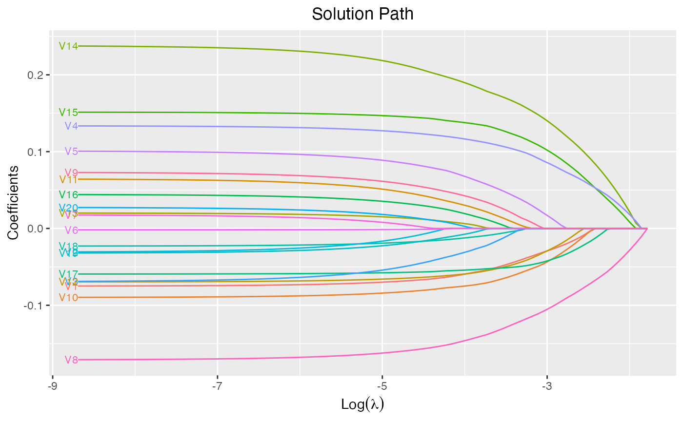
 plot(fit, xvar = "log_lambda", label = TRUE)
 fit2 <- glmtlp(X, y, family = "gaussian", penalty = "l0")
plot(fit2, xvar = "kappa", label = TRUE)
fit2 <- glmtlp(X, y, family = "gaussian", penalty = "l0")
plot(fit2, xvar = "kappa", label = TRUE)